Four canonical Odum diagrams reproduced from energese
primitives. Each is a short recipe you can copy, tweak, and adapt for
your own system.
1. El Verde tropical forest
The system Odum studied at El Verde, Puerto Rico (Odum & Pigeon 1970, funded by the U.S. Atomic Energy Commission) — the empirical basis for the entire Energy Systems Language. Sun drives an autotroph canopy; the canopy passes emergy to an understory producer + a consumer web (herbivores, decomposers); the whole loop terminates in heat.
d <- data.frame(
  x = c(1, 3.5, 6.0, 3.5, 6.0),
  y = c(3, 3.5, 3.5, 1.2, 1.2),
  role = c("Sun", "Canopy", "Understory",
           "Herbivores", "Decomposers"))

ggplot(d, aes(x, y)) +
  geom_odum_source  (data = d[1, ], radius = 0.35, fill = "#F1C40F") +
  geom_odum_producer(data = d[2, ], width = 1.4, height = 1.0,
                      fill = "#2E7D32") +
  geom_odum_producer(data = d[3, ], width = 1.4, height = 1.0,
                      fill = "#4CAF50") +
  geom_odum_consumer(data = d[4, ], width = 1.3, height = 0.9,
                      fill = "#8B4513") +
  geom_odum_storage (data = d[5, ], width = 1.3, height = 0.9,
                      fill = "#795548") +
  # Sun -> canopy, canopy -> understory
  annotate("segment", x = 1.4, xend = 2.75, y = 3, yend = 3.4,
           arrow = arrow(length = unit(0.12, "cm")), colour = ink) +
  annotate("segment", x = 4.25, xend = 5.25, y = 3.5, yend = 3.5,
           arrow = arrow(length = unit(0.12, "cm")), colour = ink) +
  # Canopy -> herbivores, understory -> decomposers
  annotate("segment", x = 3.5, xend = 3.5, y = 2.9, yend = 1.65,
           arrow = arrow(length = unit(0.12, "cm")), colour = ink) +
  annotate("segment", x = 6.0, xend = 6.0, y = 2.9, yend = 1.65,
           arrow = arrow(length = unit(0.12, "cm")), colour = ink) +
  # Decomposition loop back to canopy
  annotate("curve", x = 5.4, xend = 4.1, y = 1.2, yend = 2.9,
           curvature = 0.35, arrow = arrow(length = unit(0.12, "cm")),
           colour = "#7A6647", linetype = "dashed") +
  # Heat sinks
  geom_odum_heat_sink(data = data.frame(x = c(3.5, 6.0, 3.5, 6.0),
                                          y = c(4.9, 4.9, 0.0, 0.0)),
                       width = 0.5, height = 0.8) +
  geom_text(aes(y = y - 0.75, label = role), size = 3.2, colour = ink) +
  coord_fixed(xlim = c(0, 7.5), ylim = c(-0.9, 5.6)) +
  labs(title = "El Verde tropical forest (Odum & Pigeon 1970)") +
  theme_void() +
  theme(plot.background = element_rect(fill = bg, colour = NA),
        plot.title = element_text(hjust = 0.5, size = 12, colour = "#176b17"))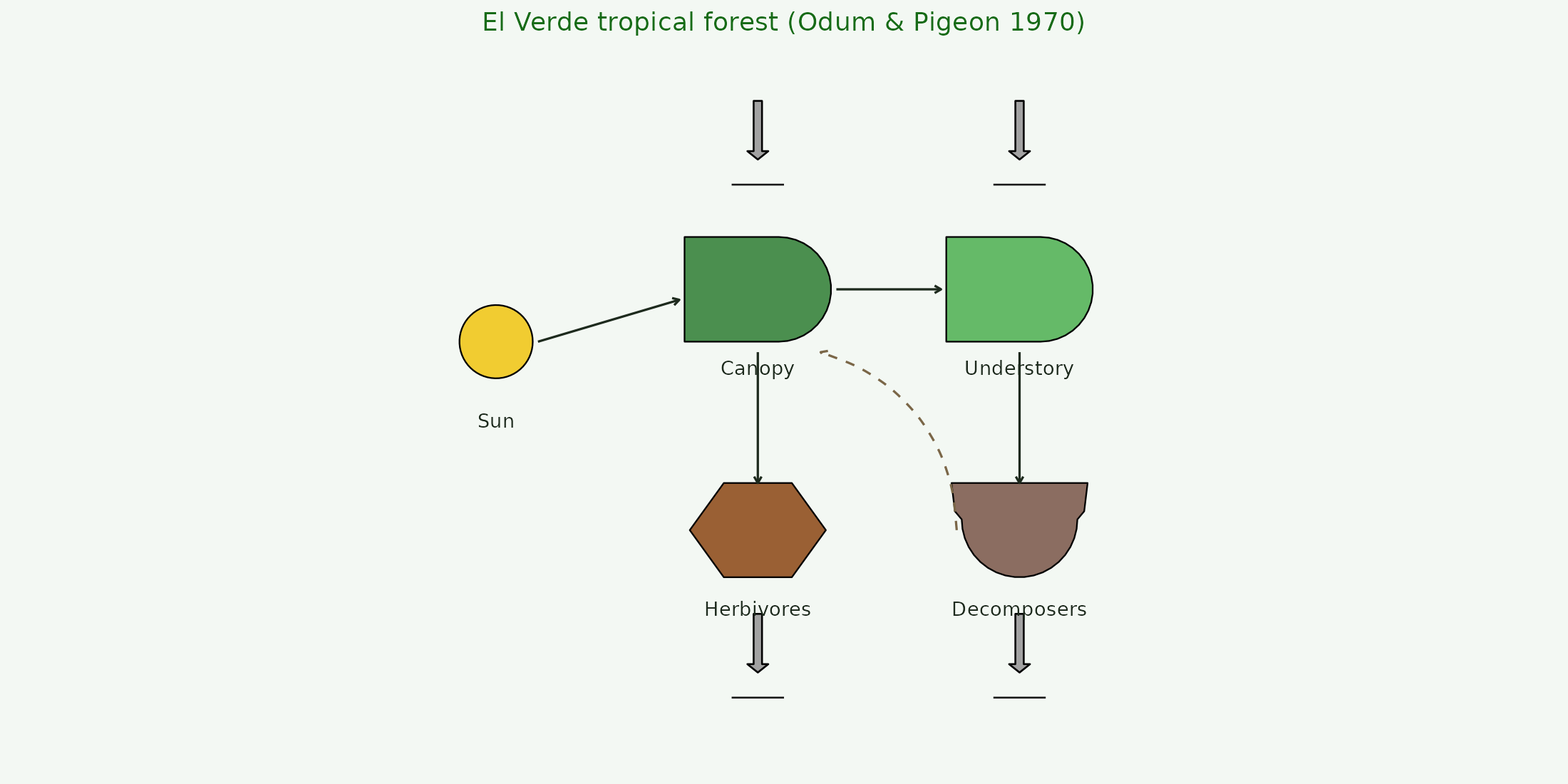
2. Urban metabolism
External fuels + food + water pass into a city consumer, which dissipates heat + waste. The classical Odum urban diagram — one consumer aggregates the entire settlement.
d <- data.frame(
  x = c(1, 1, 1, 5, 8.5),
  y = c(4, 2.5, 1, 2.5, 2.5),
  role = c("Fossil fuels", "Food", "Water", "City", "Waste + heat"))

ggplot(d, aes(x, y)) +
  geom_odum_source  (data = d[1, ], radius = 0.35, fill = "#5D4037") +
  geom_odum_source  (data = d[2, ], radius = 0.35, fill = "#2E7D32") +
  geom_odum_source  (data = d[3, ], radius = 0.35, fill = "#1976D2") +
  geom_odum_consumer(data = d[4, ], width = 1.8, height = 1.6,
                      fill = "#C0392B") +
  geom_odum_storage (data = d[5, ], width = 1.3, height = 0.9,
                      fill = "#455a64") +
  # Sources -> city
  annotate("segment", x = 1.4, xend = 4.1, y = 4,   yend = 2.9,
           arrow = arrow(length = unit(0.12, "cm")), colour = ink) +
  annotate("segment", x = 1.4, xend = 4.1, y = 2.5, yend = 2.5,
           arrow = arrow(length = unit(0.12, "cm")), colour = ink) +
  annotate("segment", x = 1.4, xend = 4.1, y = 1,   yend = 2.1,
           arrow = arrow(length = unit(0.12, "cm")), colour = ink) +
  # City -> waste
  annotate("segment", x = 5.9, xend = 7.85, y = 2.5, yend = 2.5,
           arrow = arrow(length = unit(0.12, "cm")), colour = ink) +
  # Heat sinks under the city
  geom_odum_heat_sink(data = data.frame(x = c(4.5, 5.5), y = 0.8),
                       width = 0.5, height = 0.75) +
  geom_text(aes(y = y - 0.7, label = role), size = 3.1, colour = ink) +
  coord_fixed(xlim = c(0, 10), ylim = c(-0.3, 5.2)) +
  labs(title = "Urban metabolism — one consumer, three sources") +
  theme_void() +
  theme(plot.background = element_rect(fill = bg, colour = NA),
        plot.title = element_text(hjust = 0.5, size = 12, colour = "#176b17"))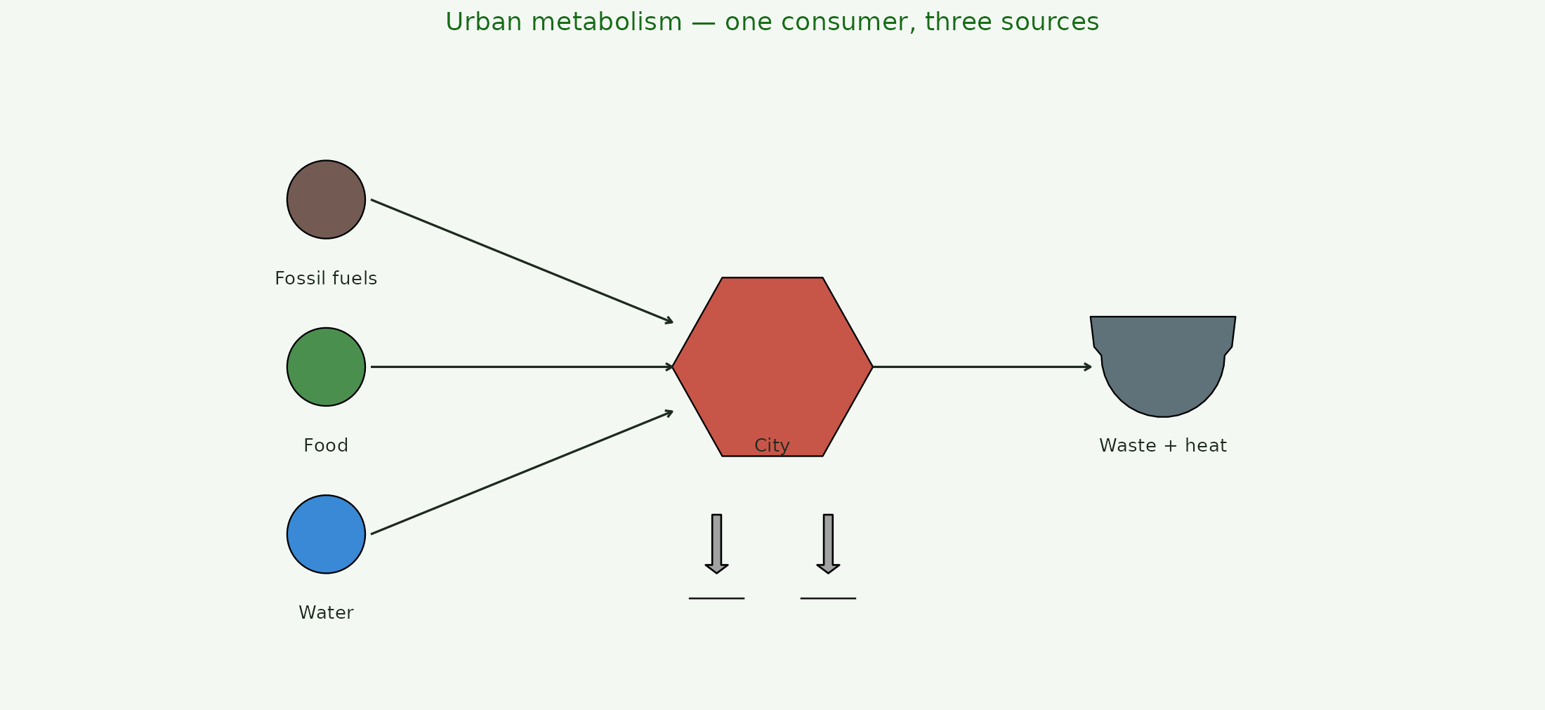
3. Ecological-economic money loop
Matter/energy flow right through the system; money flow goes counter-clockwise, left, meeting each producer and consumer at a transaction diamond. Odum used this diagram to argue for emergy-based valuation: money follows work in the opposite direction of the underlying flow it is paying for.
d <- data.frame(
  x = c(1, 3.5, 6, 8.5, 4.75, 7.25),
  y = c(3, 3, 3, 3, 1.2, 1.2),
  role = c("Sun", "Farmer", "Miller", "Baker", "$farm", "$mill"))

ggplot(d, aes(x, y)) +
  geom_odum_source     (data = d[1, ], radius = 0.35, fill = "#F1C40F") +
  geom_odum_producer   (data = d[2, ], width = 1.4, height = 1.0,
                        fill = "#2E7D32") +
  geom_odum_producer   (data = d[3, ], width = 1.4, height = 1.0,
                        fill = "#4CAF50") +
  geom_odum_consumer   (data = d[4, ], width = 1.4, height = 1.0,
                        fill = "#8B4513") +
  geom_odum_transaction(data = d[5, ], width = 1.4, height = 0.6,
                        fill = "#b5791b") +
  geom_odum_transaction(data = d[6, ], width = 1.4, height = 0.6,
                        fill = "#b5791b") +
  # Energy chain: sun -> farmer -> miller -> baker
  annotate("segment", x = 1.4, xend = 2.75, y = 3, yend = 3,
           arrow = arrow(length = unit(0.12, "cm")), colour = ink) +
  annotate("segment", x = 4.25, xend = 5.25, y = 3, yend = 3,
           arrow = arrow(length = unit(0.12, "cm")), colour = ink) +
  annotate("segment", x = 6.75, xend = 7.75, y = 3, yend = 3,
           arrow = arrow(length = unit(0.12, "cm")), colour = ink) +
  # Money counter-flow (dashed)
  annotate("segment", x = 5.5, xend = 4.0, y = 1.2, yend = 1.2,
           arrow = arrow(length = unit(0.12, "cm")),
           colour = "#b5791b", linetype = "dashed") +
  annotate("segment", x = 8.0, xend = 6.5, y = 1.2, yend = 1.2,
           arrow = arrow(length = unit(0.12, "cm")),
           colour = "#b5791b", linetype = "dashed") +
  # Transaction taps: producers <-> money
  annotate("segment", x = 3.5, xend = 4.5, y = 2.4, yend = 1.55,
           colour = "#b5791b", linetype = "dotted") +
  annotate("segment", x = 6.0, xend = 5.0, y = 2.4, yend = 1.55,
           colour = "#b5791b", linetype = "dotted") +
  annotate("segment", x = 6.0, xend = 7.0, y = 2.4, yend = 1.55,
           colour = "#b5791b", linetype = "dotted") +
  annotate("segment", x = 8.5, xend = 7.5, y = 2.4, yend = 1.55,
           colour = "#b5791b", linetype = "dotted") +
  geom_text(aes(y = y - 0.75, label = role), size = 3.1, colour = ink) +
  coord_fixed(xlim = c(0, 10), ylim = c(0.1, 3.9)) +
  labs(title = "Ecological-economic money loop",
       subtitle = "Solid = energy (rightward); dashed = money (leftward)") +
  theme_void() +
  theme(plot.background = element_rect(fill = bg, colour = NA),
        plot.title = element_text(hjust = 0.5, size = 12, colour = "#176b17"),
        plot.subtitle = element_text(hjust = 0.5, size = 9, colour = ink))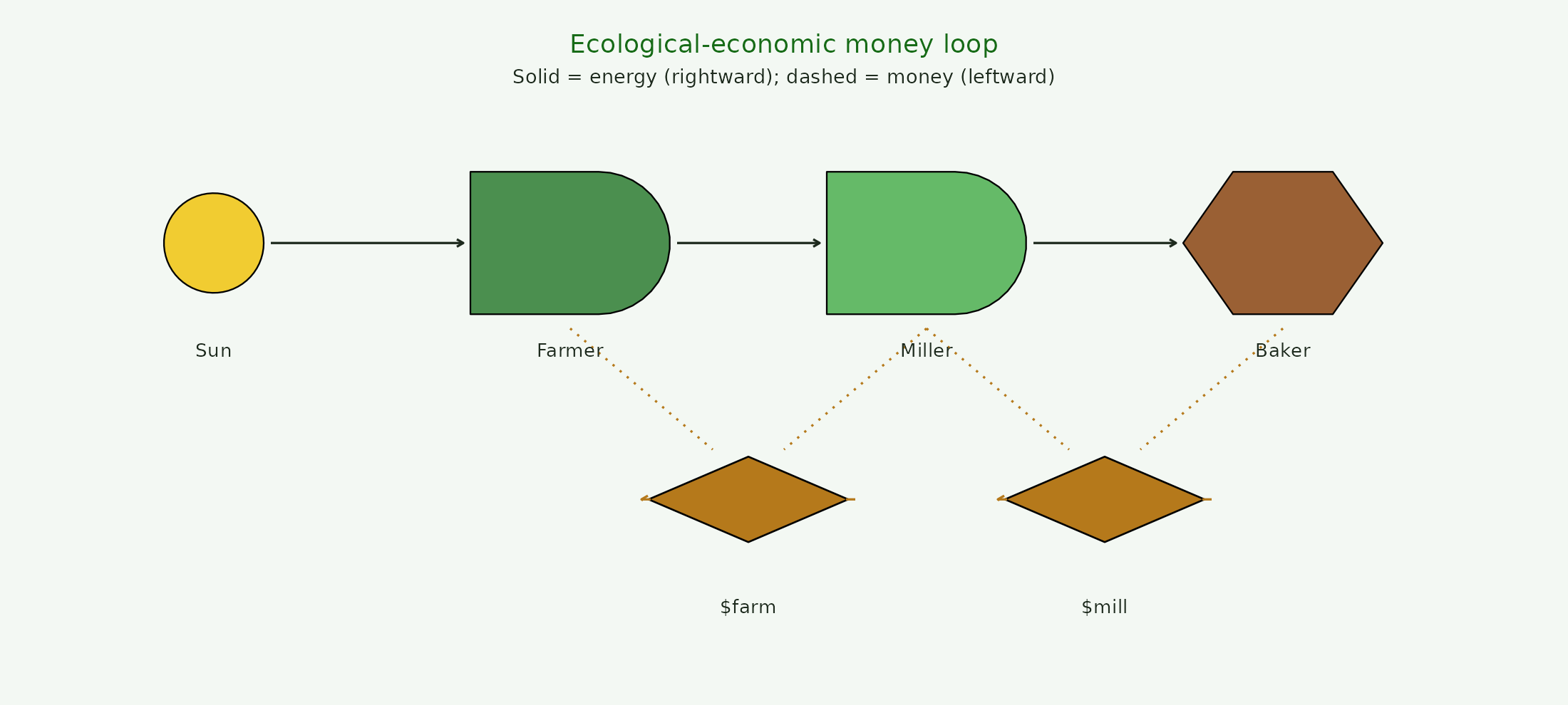
4. Aquarium / microcosm
The classroom example from Modeling for All Scales (Odum & Odum 2000): a small closed system with a source (light), a producer (algae), a consumer (fish), and a return loop through decomposition. The classic pedagogical diagram for learning to read ESL.
d <- data.frame(
  x = c(1, 4, 7, 4),
  y = c(3, 3, 3, 1),
  role = c("Light", "Algae", "Fish", "Decomposers"))

ggplot(d, aes(x, y)) +
  geom_odum_source  (data = d[1, ], radius = 0.35, fill = "#F1C40F") +
  geom_odum_producer(data = d[2, ], width = 1.4, height = 1.0,
                      fill = "#2E7D32") +
  geom_odum_consumer(data = d[3, ], width = 1.4, height = 1.0,
                      fill = "#EF6C00") +
  geom_odum_storage (data = d[4, ], width = 1.4, height = 1.0,
                      fill = "#795548") +
  annotate("segment", x = 1.4, xend = 3.25, y = 3, yend = 3,
           arrow = arrow(length = unit(0.12, "cm")), colour = ink) +
  annotate("segment", x = 4.75, xend = 6.25, y = 3, yend = 3,
           arrow = arrow(length = unit(0.12, "cm")), colour = ink) +
  annotate("segment", x = 7, xend = 4.75, y = 2.4, yend = 1.5,
           arrow = arrow(length = unit(0.12, "cm")), colour = "#7A6647",
           linetype = "dashed") +
  annotate("segment", x = 3.35, xend = 3.35, y = 1, yend = 2.5,
           arrow = arrow(length = unit(0.12, "cm")), colour = "#7A6647",
           linetype = "dashed") +
  geom_odum_heat_sink(data = data.frame(x = c(4, 7), y = 4.4),
                       width = 0.5, height = 0.75) +
  geom_text(aes(y = y - 0.75, label = role), size = 3.1, colour = ink) +
  coord_fixed(xlim = c(0, 8.5), ylim = c(0.1, 5.2)) +
  labs(title = "Aquarium microcosm (Odum & Odum 2000)") +
  theme_void() +
  theme(plot.background = element_rect(fill = bg, colour = NA),
        plot.title = element_text(hjust = 0.5, size = 12, colour = "#176b17"))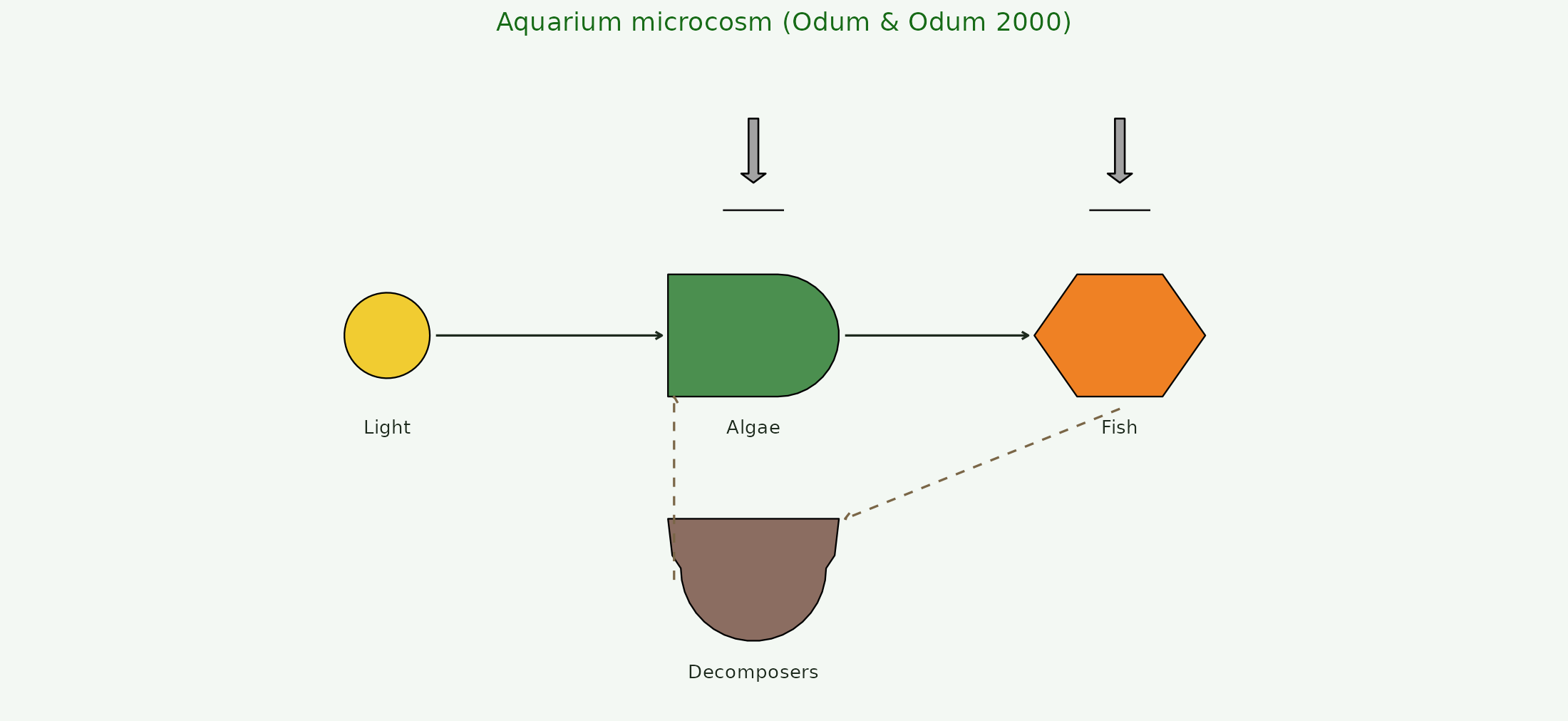
Where to go next
Each of the four diagrams above is a template. Swap the roles (source
→ wind, producer → wheat field, consumer → poultry-CAFO, storage → grain
elevator) and the whole vocabulary follows. The step-by-step vignette
(vignette("step-by-step", package = "energese")) walks
through the assembly of a single diagram one geom at a time.